Leisen-Reimer Model in Excel

This is part 6 of the Binomial Option Pricing Excel Tutorial.

So far we have implemented two binomial models in our spreadsheet: Cox-Ross-Rubinstein and Jarrow-Rudd. In this part we will extend it with another model, Leisen-Reimer.

Spreadsheet Layout

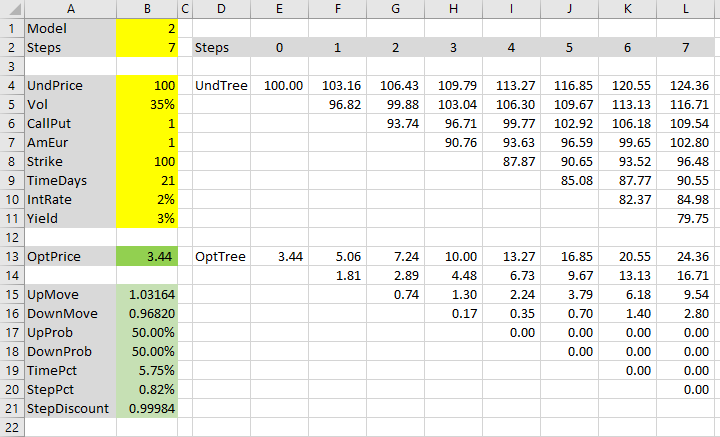
Before we start, let's make sure we start from the same point. Our spreadsheet, created in the tutorial so far, looks like this:

We have the option pricing inputs in the yellow cells B4-B11.

The green cells B15 and below calculate binomial tree parameters: up and down move sizes and probabilities.

Cell B1 selects the model to use in these tree parameter formulas. Its value is 1 for Cox-Ross-Rubinstein, 2 for Jarrow-Rudd, and now we will add 3 for Leisen-Reimer. You can as well make this cell a dropdown box.

Number of Steps

Cell B2 sets the number of steps. Its value must match the actual number of steps in the binomial trees – the underlying price tree in cells E4-L11 and option price tree in cells E13-L20.

There is one important restriction with Leisen-Reimer model:

Number of steps must be odd.

I use 7 steps throughout this tutorial; feel free to use any other number, but for Leisen-Reimer make sure it's odd. The calculations will still work with even number of steps, but they will be much less accurate.

Leisen-Reimer Model Basics

Leisen-Reimer model is newer (1995) than the other two models we have implemented. Its main advantage is that it becomes more accurate faster, with smaller number of steps. This can be particularly useful in Excel, where big binomial trees can be very slow to calculate.

When implementing the other two models, we discussed how each model has its own basic characteristic. Cox-Ross-Rubinstein has symmetric up and down moves (u · d = 1), while Jarrow-Rudd has equal up and down probabilities (50% each).

Leisen-Reimer model also has its specialty:

The underlying price tree is centered around the option's strike price at expiration, unlike the other models which tend to center the trees around the initial underlying price. This characteristic contributes to the faster convergence of Leisen-Reimer model.

It has a downside though. Besides the already mentioned odd steps restriction, the calculations of up and down moves and, particularly, probabilities, are a bit more complex in Leisen-Reimer model.

In this tutorial, we will focus mainly on Excel implementation. For detailed explanation of the model's mathematics, see Leisen-Reimer Model Formulas.

Black-Scholes d1 and d2

The first things we need to calculate is d₁ and d₂, which may be familiar from Black-Scholes model. Leisen-Reimer model uses them to calculate its probabilities.

The formulas, same as in Black-Scholes, are:

All the inputs are our option pricing inputs from cells B4-B11:

• S is underlying price (UndPrice, cell B4)
• σ is volatility (Vol, cell B5)
• K is strike price (Strike, cell B8)
• t is time to expiration in years (we have it in days in cell B9, but convert it to years in cell B19, named TimePct)
• r is risk-free interest rate (IntRate, cell B10)
• q is dividend yield (Yield, cell B11)

Let's calculate d₁ in cell B22 and define its name as BS_d1. The Excel formula is:

=(LN(UndPrice/Strike)+TimePct*(IntRate-Yield+Vol^2/2))/(Vol*SQRT(TimePct))

It is a long formula, but uses only two basic Excel functions: LN and SQRT. All the rest are our inputs (make sure you have defined all the input cell names, otherwise you will see #NAME! error).

d₂ goes in cell B23, named BS_d2:

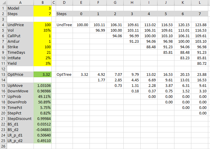
=BS_d1-Vol*SQRT(TimePct)

If you have the same inputs, you should see d₁ = 0.03512 and d₂ = -0.04883.

Peizer-Pratt Inversion

The next step is to convert Black-Scholes d₁ and d₂ to binomial probabilities, using a function called Peizer-Pratt inversion:

Good news is you don't need to remember or understand this formula to use the Leisen-Reimer model. Just write it in Excel and forget it.

It is a long formula, but takes only two arguments:

• d₁ or d₂ in place of z
• n, which is our number of steps in cell B2, named Steps

Let's calculate these inversions for d₁ and d₂ in cells B24 and B25.

The formula in cell B24 is:

=0.5+SIGN(BS_d1)/2*SQRT(1-EXP(-((BS_d1/(Steps+1/3+0.1/(Steps+1)))^2*(Steps+1/6))))

In B25 (only difference is BS_d2 in place of BS_d1):

=0.5+SIGN(BS_d2)/2*SQRT(1-EXP(-((BS_d2/(Steps+1/3+0.1/(Steps+1)))^2*(Steps+1/6))))

The results should be 0.50640 and 0.49110, respectively.

Define names for these cells as LR_p_d1 and LR_p_d2.

Leisen-Reimer Probabilities

In fact, LR_p_d2 is the up move probability in Leisen-Reimer trees.

Let's extend the UpProb (cell B17) formula to include it. The existing formula (with CRR and JR models only) is:

=IF(Model=1,
    (EXP((IntRate-Yield)*StepPct)-DownMove)/(UpMove-DownMove),
    0.5
)

It is an IF function which says: IF Model is 1 (CRR), use CRR formula, otherwise use 0.5 (the JR fixed probability).

We need to add another IF in place of the 0.5: If Model is 2 (JR), use 0.5, otherwise use LR_p_d2 (LR probability). The new formula is:

=IF(Model=1,
    (EXP((IntRate-Yield)*StepPct)-DownMove)/(UpMove-DownMove),
    IF(Model=2,
        0.5,
        LR_p_d2
    )
)

If you set cell B1 (Model) to 3, cell B17 (UpProb) should be 49.11%, same as cell B25 (LR_p_d2).

Leisen-Reimer Up and Down Move

In the same way, we will extend UpMove (cell B15) and DownMove (B16) formulas to include Leisen-Reimer model.

Leisen-Reimer up move is calculated as:

... where:

• Δt is duration of one step in years (StepPct, cell B20)
• p' is LR_p_d1 (cell B24)
• p is LR_p_d2 (cell B25)

In Excel:

=EXP((IntRate-Yield)*StepPct)*(LR_p_d1/LR_p_d2)

Make sure to put the ratio of probabilities outside the EXP.

The entire formula in cell B15, with IFs and all three models, is:

=IF(Model=1,
    EXP(Vol*SQRT(StepPct)),
    IF(Model=2,
        EXP((IntRate-Yield-Vol^2/2)*StepPct+Vol*SQRT(StepPct)),
        EXP((IntRate-Yield)*StepPct)*(LR_p_d1/LR_p_d2)
    )
)

Down move is:

In Excel:

=EXP((IntRate-Yield)*StepPct)*((1-LR_p_d1)/(1-LR_p_d2))

So the formula in cell B16 is:

=IF(Model=1,
    1/UpMove,
    IF(Model=2,
        EXP((IntRate-Yield-Vol^2/2)*StepPct-Vol*SQRT(StepPct)),
        EXP((IntRate-Yield)*StepPct)*((1-LR_p_d1)/(1-LR_p_d2))
    )
)

Option Price

Now we have all the Leiser-Reimer tree parameters correct and our spreadsheet works for all three models.

The resulting option price (cell B13) is 3.3178, considerably less than the 3.44 we got under either CRR and JR model.

In fact, the Leisen-Reimer price is much closer to reality. If you priced the same option with 101 steps, the models would return 3.3184 (LR), 3.3228 (JR) and 3.3267 (CRR).

Leisen-Reimer model needs very few steps to calculate very precise option prices. Seven may still be a bit low for practical use, but somewhere around 20 (must be odd!) should be more than enough in most cases.

Conclusion and Things to Improve

This is the end of the Binomial Option Pricing Excel Tutorial. We have a spreadsheet which can be used to price various options (American, European, calls, puts, options on stocks, indexes or currencies) with three different models.

There are still things we could add or improve.

Dropdown Boxes

For instance, some of our inputs would be more user-friendly as dropdown boxes rather than typed values: namely Model, CallPut, AmEur.

Variable Steps

We could also make the tree size dynamic. By adding some IFs to the formulas inside the trees, we could change tree size merely by changing the value in cell B2 (Steps).

If you choose to make this adjustment, keep in mind that the last step in option price tree contains different formulas (payoffs at expiration) than the other steps. You can easily handle that with IFs: IF step number in row 2 equals the value of Steps cell, use payoff formula etc.

More Features

With small adjustments, we could make our spreadsheet also work with futures options.

Or (with bigger adjustments) with discrete dividends.

Greeks

While you could get estimates of delta, gamma, and (under CRR model) theta directly from the binomial trees, other Greeks can't be calculated directly and require another instance of binomial trees (incrementing the particular input, e.g. volatility for vega). This is better to do with VBA than plain Excel.

Chart

Another desirable feature would be a chart, drawing option price as function of a selected input, like underlying price.

Unfortunately, this also requires VBA, which is beyond the scope of this tutorial. Moreover, even with VBA, it can cause serious performance issues with more than a small number of steps (basically you need to rebuild the entire trees for every point in the chart series). It can be done, but you should pay maximum attention to computational efficiency (intermediate calculations, not calculating the same thing more than once etc.).

I have implemented charts, Greeks and the other listed features in the Binomial Option Pricing Calculator.

If you have any comments or feedback, please feel free to contact me.