Creating Binomial Trees in Excel

This is part 3 of the Binomial Option Pricing Excel Tutorial.

In the first part we have prepared and named our input cells. In the second part we have explained how binomial trees work. In this part we will create underlying price tree and option price tree in our spreadsheet.

Up and Down Move Sizes and Probabilities

In the previous part we have explained that main parameters needed for building a binomial tree are up and down move sizes and probabilities:

• From each node, price can go up or down.
• These move sizes and probabilities are constant throughout the tree.
• They can be different for up and down moves.
• The probabilities must add up to 100%.

Move sizes and probabilities are calculated from model inputs, like interest rate and volatility, which we have prepared in cells B4-B11.

The formulas for up and down move sizes and probabilities are different in different binomial models, but everything else – structure and all formulas inside the binomial trees – are the same in all the models.

Therefore, we will first use dummy values for our move sizes and probabilities, create the trees first with these dummy values, and in the next parts of the tutorial we will replace these values with correct formulas for individual models (Cox-Ross-Rubinstein, Jarrow-Rudd, and Leisen-Reimer).

For now, let's assume up and down move sizes are +1% and -1%, respectively, and their probabilities are 50% each. Put them in cells B15-B18.

The move sizes are expressed as 1 + the percentage, that is 1.01 for the +1% up move and 0.99 for the -1% down move.

Let's name the cells UpMove, DownMove, UpProb, DownProb. Register the cell names in Excel using one of the methods introduced in part 1 (you can also right click the cell and select "Define Name"). This will allow us to use these names in formulas, which makes our formulas easier to write and understand.

Now we can start creating the actual trees. The first task is to decide their layout.

Choosing the Best Tree Layout for Excel

On paper a binomial tree may look like this:

In Excel, you can shape it in three ways:

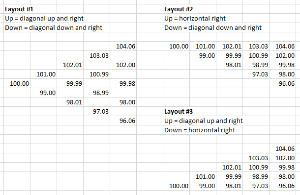
I recommend layout #2, for two reasons:

1. The first node is in the top row.
2. There are no empty cells inside the tree.

Both make inserting and maintaining formulas, or resizing the tree, much easier.

If you are creating trees with many steps, it is best to put each tree in its own sheet (with matching columns and rows for same steps and nodes). In this tutorial we are creating trees with only 7 steps, so we will put both in one sheet, next to our input cells.

Let's create the underlying price tree first.

Underlying Price Tree

Inputs for this tree are:

• Current underlying price (cell B4 named UndPrice)
• Up and down price move sizes (cells B15-B16 named UpMove, DownMove)

The first node, which equals current underlying price, will be in cell E4. The formula is very simple:

=UndPrice

Up and Down Move Formulas

Choosing #2 from the three layouts introduced above, our tree will have up moves horizontal (next cell to the right) and down moves diagonal (down and right). Therefore, if price moves up in the first step (from cell E4), it will end up in cell F4. The formula is:

=E4*UpMove

Down move from the initial cell E4 takes us to cell F5. The formula is:

=E4*DownMove

We have just created a one-step binomial tree.

Adding Steps

Extending it to more steps is very simple, because the formulas stay the same throughout the tree. We can just copy them (make sure the references to E4 are relative in the above formulas – no dollar signs).

Our 7-step tree will be 8 columns wide, because the initial node is not considered a step. Let's label the steps in row 2. Feel free to create as many steps as you want.

Each additional step will have one node more than the previous step. In each subsequent column, add a node at the bottom – a down move from the previous column's bottom node.

Because a * b = b * a, or in our case up * down = down * up, it doesn't matter whether a node is calculated as an up move from the node to the left, or as down move from the node to the left and up – both give the same result. It is best to be consistent though – I copy the up move formulas in the top row only, and use the down move formulas elsewhere.

That's it. We have created the underlying price tree.

Option Price Tree

The last column in the underlying price tree contains different underlying prices at expiration. We will use them to calculate option payoffs at expiration for these different scenarios, which will be the last column in the option price tree.

Remember from the previous part: While underlying price tree is calculated from left to right, option price tree is calculated backwards – from right to left, or from payoffs at expiration to current option price.

Payoff at Expiration

Let's create our option price tree below the underlying price tree, in row 13 and below.

Cell L13 calculates option payoff at expiration for the underlying price in cell L4:

=MAX(0,IF(CallPut=1,L4-Strike,Strike-L4))

Payoff at expiration is different for calls and puts. If our CallPut cell contains the value 1, the option is a call, otherwise a put. Call payoff is underlying price at expiration (cell L4) minus strike; put payoff is strike minus underlying price. If these differences are negative (option expires out of the money), payoff is zero, which is done with the MAX function. More explanation here.

Make sure the reference to L4 is relative (no dollar signs). Copy the formula from cell L13 to the seven cells below (L14-L20).

If your inputs match mine, you should see the four upper cells L13-L16 showing positive values 7.21, 5.09, 3.01, 0.97, respectively, which is the underlying prices from cells L4-L7 minus strike price (all cells are rounded to two decimal places). The bottom cells L17-L20 show zero, because the related underlying prices in cells L8-L11 are below the strike price and the call option expires out of the money (if you changed the CallPut input cell to 2, it would be the opposite).

We have created the last step in our option price tree. Now we will calculate the earlier steps, moving from right to left.

Earlier Nodes

What will be the option price in cell K13?

It is the top node in the penultimate step (one step before expiration).

There are only two possible paths from this cell to the last step – either underlying price goes up and option price (payoff at expiration) will be 7.21 (cell L13), or underlying price goes down and option price will be 5.09 (cell L14).

We also know the probabilities: 50% to each.

We know all we need to calculate expected value of the option: If there is 50% chance option price will be 7.21 and 50% chance it will be 5.09, expected value is the weighted average, using the probabilities as weights. The formula in K13 becomes:

=(L13*UpProb+L14*DownProb)

It is not finished though.

Step Discount

Recall from the previous part of the tutorial that the above formula is the option's expected value at the next step, but we need its present value. Therefore we need to discount it – multiply it by the discount factor:

... where r is the IntRate input (cell B10) and Δt is step duration in years, or time to expiration divided by number of steps.

For better performance (especially when working with high number of steps) it is best to calculate this discount factor in a separate cell, instead of calculating it repeatedly in each option price tree cell.

Let's calculate the discount factor it in cells B19-B21.

First, set up a new input cell B2 and name it Steps. Enter number of steps, in our case 7.

Cell B19, which we will name TimePct, calculates time to expiration in years. Our TimeDays input in cell B19 is time to expiration in days, so we need to divide it by 365:

=TimeDays/365

Cell B20 (StepPct) calculates step duration in years – it divideds B19 by the number of steps:

=TimePct/Steps

Finally, cell B21 (StepDiscount) calculates the step discount factor, using the EXP function:

=EXP(-IntRate*StepPct)

Now we can update our option price formula in cell K13, adding the discount factor (make sure you have registered the name StepDiscount for cell B21):

=(L13*UpProb+L14*DownProb)*StepDiscount

Cell K13 now shows the correct European option price (with our inputs it should be 6.151004).

American Options and Early Exercise

To make our spreadsheet work also for American options, we need to add a bit more logic to the formula in cell K13: We need to check whether it's profitable to exercise the option early (see detailed explanation of the logic).

In other words, the new option price is the greater of:

• The European option price we have just calculated.
• The option's intrinsic value (what we would get from exercising) if the option is American, or zero if it's European (exercise not possible).

In Excel we can do this using MAX and IF functions. The new formula in cell K13 will be:

=MAX((L13*UpProb+L14*DownProb)*StepDiscount,... second item ...)

There are two items inside the MAX function. The first is the old European option formula.

The second item is:

IF(AmEur=1,IF(CallPut=1,K4-Strike,Strike-K4),0)

It is a nested IF function. The outer IF uses our AmEur input as condition. If the option is American (AmEur is 1), the second item in the MAX is the option's intrinsic value (the inner IF). Otherwise (AmEur is not 1), it is zero.

Intrinsic value is calculated as:

IF(CallPut=1,K4-Strike,Strike-K4)

If the option is a call (CallPut is 1), intrinsic value is underlying price minus strike. Otherwise (CallPut is not 1), it is strike minus underlying price. Two notes:

• Underlying price in this formula is not the initial underlying price (UndPrice input cell), but a node from the underlying price tree – in this case cell K4. Make sure to use relative reference.
• We don't need to add MAX(0,...) to this intrinsic value calculation as we normally would, because the result is already inside a MAX, being compared to a value which is never negative (the European option price).

The entire, final formula for the option price in cell K13 is:

=MAX((L13*UpProb+L14*DownProb)*StepDiscount,IF(AmEur=1,IF(CallPut=1,K4-Strike,Strike-K4),0))

The result with our inputs is 6.152015 – slightly greater than our previous result (6.151004) before the American option adjustment. In this particular case, at this node, American option should be exercised, because its intrinsic value 6.152 is greater than its expected value 6.151. The difference is $0.001 though – not material in practice.

Completing the Tree

Now we can copy the formula from K13 to all remaining nodes in the option price tree. It must have the same shape as the underlying price tree, and the intrinsic value formulas must refer to the underlying price tree nodes at the exact same locations.

The first node (cell E13) is the current option price, the ultimate output. We can set cell B13 equal to E13.

Next: Move Sizes and Probabilities

We have completed the binomial trees – the part that is common for all the models. But our spreadsheet is not done yet, because we have used dummy values for up and down move sizes and probabilities. Their calculation is different under different binomial models.

In this tutorial I will introduce three of the most popular models:

• Cox-Ross-Rubinstein
• Jarrow-Rudd
• Leisen-Reimer

If you are only interested in one of them, feel free to skip the other parts.

Otherwise I recommend doing them in this order (Leisen-Reimer calculations are a bit more complex, so we will do them last).

Let's start with the best known binomial option pricing model: Cox-Ross-Rubinstein.