This page explains the logic of binomial option pricing models – how option price is calculated from the inputs using binomial trees, and how these trees are built.
Binomial Model Assumptions
All models simplify reality, in order to make calculations possible, because the real world (even a simple thing like stock price movement) is often too complex to describe with mathematical formulas.
Binomial option pricing models make the following assumptions.
Discrete Steps
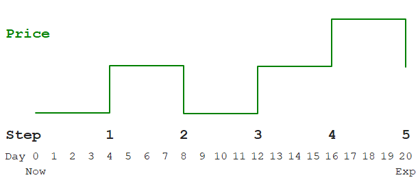
Prices don't move continuously (as Black-Scholes model assumes), but in a series of discrete steps.
Time between steps is constant and easy to calculate as time to expiration divided by the model's number of steps.
For example, if you want to price an option with 20 days to expiration with a 5-step binomial model, the duration of each step is 20/5 = 4 days. Once every 4 days, price makes a move.
Up and Down Moves
At each step, the price can only do two things (hence binomial): Go up or go down.
The sizes of these up and down moves are constant (percentage-wise) throughout all steps, but the up move size can differ from the down move size.
For instance, at each step the price can either increase by 1.8% or decrease by 1.5%. These exact move sizes are calculated from the inputs, such as interest rate and volatility.
Like sizes, the probabilities of up and down moves are the same in all steps. They must sum up to 1 (or 100%), but they don't have to be 50/50. Like sizes, they are calculated from the inputs.
For example, from a particular set of inputs you can calculate that at each step, the price has 48% probability of going up 1.8% and 52% probability of going down 1.5%.
This is all you need for building binomial trees and calculating option price.
How to Calculate Option Price
These are the things to do (not using the word steps, to avoid confusion) to calculate option price with a binomial model:
- Know your inputs (underlying price, strike price, volatility etc.).
- From the inputs, calculate up and down move sizes and probabilities.
- Build underlying price tree from now to expiration, using the up and down move sizes.
- The final step in the underlying price tree shows different underlying prices at expiration for different scenarios.
- From the above, calculate option payoff at expiration for different scenarios = the final step in the option price tree.
- Build the option price tree backwards from expiration to now.
- The price at the beginning of the option price tree is the current option price.
Underlying Price Tree
We have already explained the logic of points 1-2. Exact formulas for move sizes and probabilities differ between individual models (for details see Cox-Ross-Rubinstein, Jarrow-Rudd, Leisen-Reimer). The rest is the same for all models.
For now, let's use some round values to explain how binomial trees work:
- Up and down move sizes +1% and -1%
- Probabilities 50% each
- Current underlying stock price $100
The simplest possible binomial model has only one step. A one-step underlying price tree with our parameters looks like this:
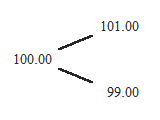
It starts with current underlying price (100.00) on the left. From there price can go either up 1% (to 101.00) or down 1% (to 99.00).
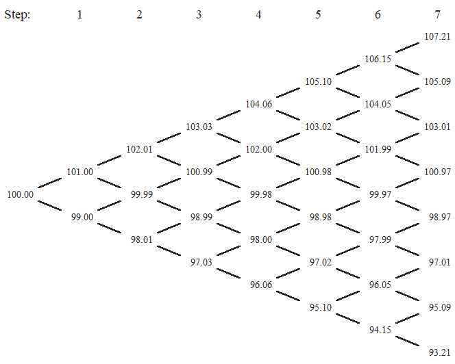
There is no theoretical upper limit on the number of steps a binomial model can have. Generally, more steps means greater precision, but also more calculations. In this tutorial we will use a 7-step model.
Binomial Tree Characteristics
Individual steps are in columns.
The first column, which we can call step 0, is current underlying price.
In each successive step, the number of possible prices (nodes in the tree), increases by one.
The number of nodes in the final step (the number of possible underlying prices at expiration) equals number of steps + 1.
There are two possible moves from each node to the next step – up or down.
There are also two possible moves coming into each node from the preceding step (up from a lower price or down from a higher price), except nodes on the edges, which have only one move coming in.
Calculating the Tree
Knowing the current underlying price (the initial node) and up and down move sizes, we can calculate the entire tree from left to right.
Each node can be calculated either by multiplying the preceding lower node by up move size (e.g. by 1.02 if up move is +2%), or by multiplying the preceding higher node by down move size. Both should give the same result, because a · b = b · a.
Paths and Probabilities
There can be many different paths from the current underlying price to a particular node. For instance, up-up-down (green), up-down-up (red), down-up-up (blue) all result in the same price, and the same node.
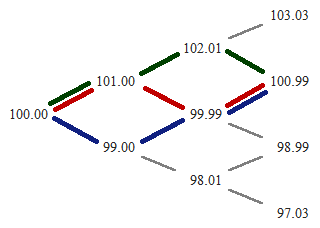
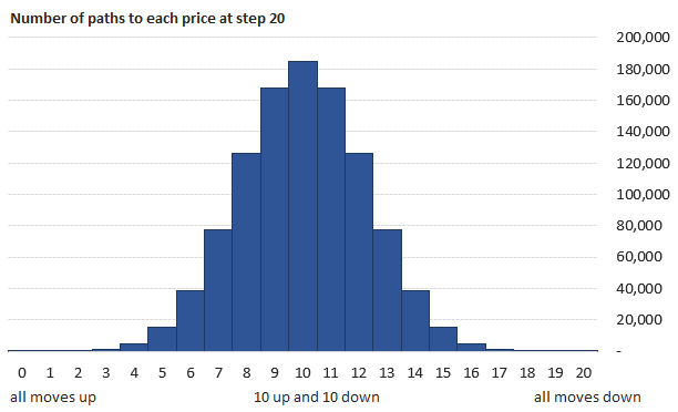
Notice how the nodes around the (vertical) middle of the tree have many possible paths coming in, while the nodes on the edges only have a single path (all ups or all downs). This reflects reality – it is more likely for price to stay the same or move only a little than to move by an extremely large amount.
If you are thinking of a bell curve, you are right. With growing number of steps, number of paths to individual nodes approaches the familiar bell curve.
Option Payoff at Expiration
The last step in the underlying price tree gives us all the possible underlying prices at expiration. For each of them, we can easily calculate option payoff – the option's value at expiration.
Two things can happen at expiration.
If the option ends up in the money, we exercise it and gain the difference between underlying price S and strike price K:
If the above differences (potential gains from exercising) are negative, we choose not to exercise and just let the option expire. The option's value is zero in such case.
Therefore, option value at expiration is:
C = max(0, S – K)
P = max(0, K – S)
These option values, calculated for each node from the last column of the underlying price tree, are in fact the option prices in the last column of the option price tree.
Option Price Tree
While underlying price tree is calculated from left to right, option price tree is calculated backwards – from the set of payoffs at expiration, which we have just calculated, to current option price.
Each node in the option price tree is calculated from the two nodes to the right from it (the node one move up and the node one move down).
We already know the option prices in both these nodes (because we are calculating the tree right to left).
We also know the probabilities of each (the up and down move probabilities).
With all that, we can calculate the option price as weighted average, using the probabilities as weights:

... where Ou and Od are option prices at next step after up and down move, and
p is probability of up move (therefore 1 – p must be probability of down move).
But we are not done. We must discount the result to account for time value of money, because the above expression is expected option value at next step, but we want its present value, one step earlier. The discount factor is:

... where r is the risk-free interest rate and Δt is duration of one step in years, calculated as t/n, where t is time to expiration in years (days to expiration / 365), and n is number of steps.
The formula for option price in each node (same for calls and puts) is:

Using this formula, we can calculate option prices in all nodes going right to left from expiration to the first node of the tree – which is the current option price, the ultimate output.
American Options and Early Exercise
The above formula holds for European options, which can be exercised only at expiration. This is why I have used the letter E, as European option or expected value if we hold the option until next step.
American options can be exercised early. We must check at each node whether it is profitable to exercise, and adjust option price accordingly.
American option price will be the greater of:
- What we would gain from exercising
- The option's expected value when not exercising = E
We need to compare the option price E with the option's intrinsic value, which is calculated exactly the same way as payoff at expiration:
C = max(0, S – K)
P = max(0, K – S)
... where S is the underlying price tree node whose location is the same as the node in the option price tree which we are calculating.
If intrinsic value is higher than E, the option should be exercised. Option price equals the intrinsic value.
Otherwise (it is not profitable to exercise, so we keep holding the option) option price equals E.
This is probably the hardest part of binomial option pricing models, but it is the logic that is hard – the mathematics is quite simple.
When implementing this in Excel, it means combining some IFs and MAXes:
- IF the option is American, option price is MAX of intrinsic value and E.
- Otherwise (it's European) option price is E.
- IF the option is a call, intrinsic value is MAX of zero and S – K.
- Otherwise (it's a put) intrinsic value is MAX of zero and K – S.
We will create both binomial trees in Excel in the next part.