When you work with time series in Excel and import data from sources which use different date format than your operating system, Excel sometimes loads the dates incorrectly. It may swap day and month or not recognize the expression as date and treat it as text.
The first solution to try is the Text to Columns feature - it's quick and easy; it often works, but sometimes it doesn't. In such cases you can usually fix the dates using formulas which combine various date and text Excel functions.
In this short tutorial I will show you both these solutions.
Example of the Reverse Date Problem
My computer is set to work with dates in the "d/m/yyyy" (UK) format, but I often work with historical financial data in the US format "m/d/yyyy". For example, I may download the VIX index historical data from the CBOE website (direct file link here) - the current version is a CSV file which starts like this:
Date,VIX Open,VIX High,VIX Low,VIX Close
1/2/2004,17.96,18.68,17.54,18.22
1/5/2004,18.45,18.49,17.44,17.49
1/6/2004,17.66,17.67,16.19,16.73
1/7/2004,16.72,16.75,15.5,15.5
It contains the daily open, high, low, close for the VIX index, starting from January 2004.
When I load this file in Excel, it looks like this:
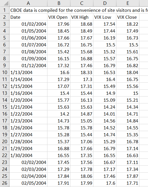
My computer, which is looking for "d/m/yyyy" dates has no way to know that this particular CSV file stores dates in the "m/d/yyyy" format. As a result, 2 January becomes 1 February, 5 January becomes 1 May and so on - the day and month have been reversed.
Moreover, once you get to 13 January (row 10), Excel no longer treats the expressions as dates, because there is no 13th or 14th month.
In sum, in the Date column you end up with two kinds of cells:
- Incorrect dates with reversed day and month (for rows where the original date has day <= 12)
- Text (for rows where the original day, which Excel thinks should be a month > 12)
This must be fixed before you can do any meaningful work with the data.
Text to Columns Solution
For those not familiar with the Text to Columns feature, let me first mention that one, because when it works, it is much faster than converting the dates using some formulas you build. It is worth trying first.
Select the column with dates and go to Excel main menu / Data / Text to Columns.
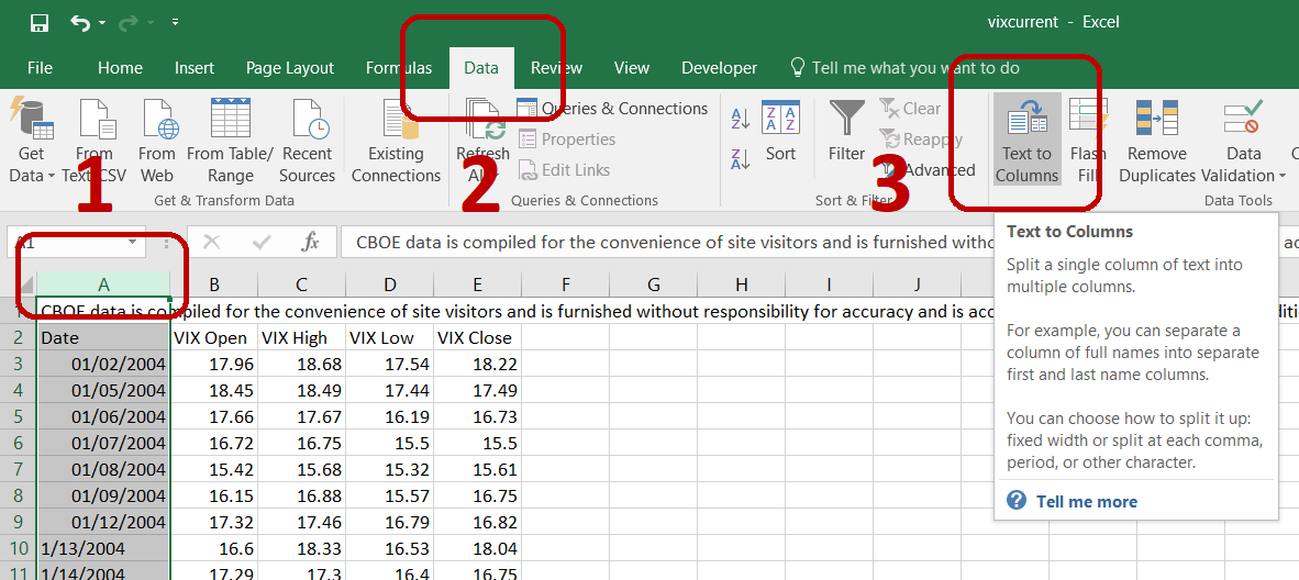
A window pops up and you will go through three steps. The first two steps let you decide whether your data is delimited and what the delimiter characters are - these are not important when having only one column selected. The important thing happens in step 3, where you can select the data format.
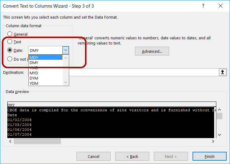
Check Date and select the format that you think matches the original data source (e.g. MDY if the dates in the original CSV file are something like "m/d/yyyy"). Click Finish and see if the dates have been fixed.
Unfortunately, sometimes this simple solution doesn't work and it's time for the harder, formula-based fix, which I introduce below.
Manual Formula-Based Solution
We will create a formula to calculate correct dates from the incorrect ones, of which:
- some are dates with reversed day and month, e.g. 1 February, which we must convert to 2 January
- some are text not recognized as date, e.g. "1/13/2004" (text), which we must convert to 13 January (date)
Before we start, let's save the spreadsheet as an Excel file (xlsx or xls), which will enable us to save formulas and formats which a CSV can't store.
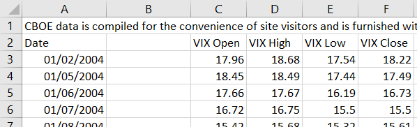
Insert a new column before column B. We will calculate the correct dates in this column.
Fixing the Reverse Day and Month Cells
The first kind of cells (e.g. in rows 3-9 in our example) are recognized as dates in Excel, only with reverse order of day and month. Therefore we can extract the day, month, and year piece using the functions DAY, MONTH, and YEAR, respectively. Only thing to remember is that the result of DAY is really the month in our case and the result of MONTH is the day.
Then we can combine the individual pieces into a correct date, using the DATE Excel function, which takes three arguments: year, month, day - in this order - and returns a date.
In cell B3, let's calculate the correct date for the first row (which should be 2 January 2004, but cell A3 is 1 February 2004).
The formula in cell B3 is:
=DATE(YEAR(A3),DAY(A3),MONTH(A3))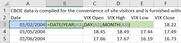
... where:
YEAR(A3)is 2004DAY(A3)is 1, becauseA3is 1 FebruaryMONTH(A3)is 2
... so the values of our DATE arguments are:
=DATE(2004,1,2)... which returns the correct date: 2 January 2004.
Fixing the Text Cells
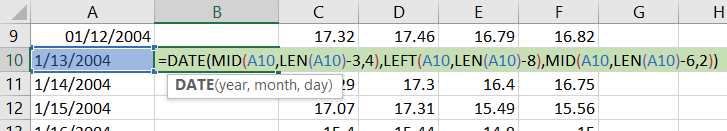
The other kind of cells (e.g. rows 10 and below in our example) are not recognized as dates in Excel, because the day (treated as month) is greater than 12 and there is of course no 13th month.
For instance, in cell A10 we have the text "1/13/2004" which we want to convert to the date 13 January 2004.
We will do that using the DATE function again, but this time we must get the three arguments - year, month, day - differently. We must extract them as pieces of the text, using Excel functions LEFT and MID.
Getting Month Using LEFT
The LEFT function extracts the beginning of a string from the first character up to and including the n-th character. It takes two arguments: the original text and the position of the last character to include. Therefore, if we want to get the month from cell A10 (get the "1" from "1/13/2004"), the formula is:
=LEFT(A10,1)It means: get the first (one) character from the text in cell A10.
Unfortunately, this only works for months 1-9. For dates where the month has two digits (for example, the text is "10/13/2004" = 13 October 2004), we in fact need the formula:
=LEFT(A10,2)Therefore, we need to make the second argument of the LEFT function dynamic.
We can calculate the desired number of characters (1 for months 1-9 or 2 for months 10-12) by subtracting 8 from the length of the entire string (using the LEN Excel function). The rest of the string after the month has always the same length - 8 characters: "/dd/yyyy". The day always has two characters, because dates with day 1-12 all go to the first type of cells which we have already fixed above.
The dynamic formula for extracting the month from cell A10 is:
=LEFT(A10,LEN(A10)-8)... where the result of LEN(A10)-8 is 1 for single digit months and 2 for months 10-12.
Getting Day and Year Using MID
Unlike month, day and year can't be obtained using the LEFT function, because they start in the middle of the string. We will use the Excel function MID, which takes three arguments:
=MID(original text, position of first character to return, number of characters)For example, if we want to get the number 13 (the third and fourth character) from the string "1/13/2004" in cell A10, the formula is:
=MID(A10,3,2)However, we must make the second argument (starting position) dynamic to work for both single digit and double digit months.
We can use the LEN function again. The first character of day can be calculated as length of the string minus 6. The six characters after that are always "d/yyyy" where d is the second character of day.
The formula for extracting day from cell A10 is:
=MID(A10,LEN(A10)-6,2)... where LEN(A10)-6 equals 3 for single digit months and 4 for months 10-12.
We can get year in the same way, this time subtracting 3 from LEN, because the remaining characters after the first character of year are always "yyy":
=MID(A10,LEN(A10)-3,4)The third argument is now 4, because year always has 4 characters.
Getting the Date
The last step for getting correct date from the text cells is to combine day, month and year using the DATE function. The formula in cell B10 is:
=DATE(MID(A10,LEN(A10)-3,4),LEFT(A10,LEN(A10)-8),MID(A10,LEN(A10)-6,2))where:
MID(A10,LEN(A10)-3,4)is the yearLEFT(A10,LEN(A10)-8)is the monthMID(A10,LEN(A10)-6,2))is the day
Note: We are calculating the same thing (the LEN) three times in this formula. If you are working with a very large dataset and performance is an issue, you may want to calculate the LEN in a different column and plug that column into this formula. For small files our solution is OK.
Combining the Two Types
We have fixed both types of cells and we can now combine the formulas into one universal solution that would work for all rows. We can use the IF function:
=IF(condition, result when true, result when false)To check the type of cell, we will use the ISNUMBER function, which takes one argument and returns TRUE if the argument is a value treated as number in Excel, and FALSE otherwise.
All dates are in fact numbers in Excel, just displayed with formatting that makes them appear as dates to humans. Try to change the Number Format for a date in Excel. For example, you will find that 2 January 2004 is actually the number 37,988. Number 1 is 1 January 1900.
We will construct our IF function like this:
If the cell in column A is the first type (ISNUMBER returns TRUE), use the formula for the first type, otherwise use the second type.
The combined formula in cell B3 is:
=IF(ISNUMBER(A3),DATE(YEAR(A3),DAY(A3),MONTH(A3)),DATE(MID(A3,LEN(A3)-3,4),LEFT(A3,LEN(A3)-8),MID(A3,LEN(A3)-6,2)))... plugging in the formulas for both types which we have developed.
You can now copy this formula to all rows in column B and paste them as values. You should see the correct dates.
You may want to delete the original incorrect dates column if your file is very big and performance is an issue, but in any case I recommend also keeping the original data file, just in case you discover any errors going forward.
Our solution assumes the date format in the original CSV file, while not correctly recognized by our computer, is correct by itself. Sometimes that is unfortunately not true. You may have special characters next to dates in some rows, such as a star ("9/17/2015*" denoting a comment or special situation on that date). This could be a problem for our LEN function. In some cases the date format is inconsistent across the file (e.g. the file starts with "mm/dd/yyyy" but suddenly switches to "m.d.yy" midway). These should of course be checked before doing any work.
The End
In this tutorial I have shown you how to fix some of the common issues which may arise from regional differences in date formatting (personally I do these things more often than I would like to).
I hope you have found it useful, either for fixing a particular problem you're facing, or for learning a bit about date and text manipulation in Excel.
If you have any questions or suggestions, perhaps you are using a different solution which may be better in some cases, please feel free to send me a message.