This is the second part of the Average True Range (ATR) Excel tutorial. In the first part we have calculated ATR using the simple moving average method. Now we will calculate ATR using two other popular methods – exponential moving average and Wilder's smoothing method.
First Part Recap (SMA ATR)
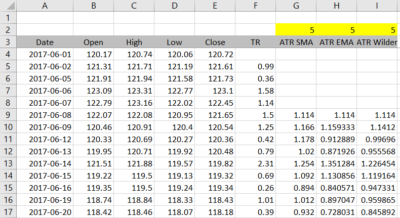
From the first part we have a spreadsheet with historical data in columns A-E, true range in column F and SMA ATR in column G.
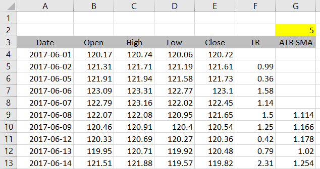
Now we will calculate exponential moving average ATR in column H.
Exponential Moving Average ATR
This method calculates ATR as exponential moving average of true range, in the same way exponential moving average of closing price works.
Each bar's ATR is calculated as weighted average of two inputs:
- The current bar's true range
- The previous bar's ATR
The formula is:
ATR = a · TR + ( 1 – a ) · ATR1
... where TR is current bar's true range, ATR1 is previous bar's ATR and a is the smoothing factor, which is calculated from the ATR period input (n):
a = 2 / ( n +1 )
For example, when you set ATR period to 14, the smoothing factor will be:
a = 2 / ( 14 + 1 ) = 2 / 15 = 0.1333
... and each bar's ATR will be:
ATR = 0.1333 · TR + 0.8667 · ATR1
In other words, ATR will be composed of roughly 13% of current bar's true range and 87% of previous bar's ATR. These weights will change with ATR period – the shorter the period, the greater the weight of current bar's true range and the faster ATR reacts to changing market conditions.
There is one problem though. When each bar's ATR is calculated using the previous bar's ATR, how do we calculate ATR for the first bar? The answer is arithmetic average – exactly the same we did in the SMA method calculation (this is why the tutorial does the SMA method first).
Excel Implementation of EMA ATR
Let's place ATR period input in cell H2 in our spreadsheet.

The formulas in column H will use IF Excel functions and perform three different calculations, based on which row it is:
- In the first n rows (where n is the ATR period) there is not enough data for ATR calculation, so the formula should return "" – empty cell (alternatively you can set it to return #N/A or something else).
- In the n+1'th row calculate arithmetic average of true range from all rows up to this one.
- In all the subsequent rows, calculate ATR from previous row's ATR and current row's true range, using the formula explained above.
IF Conditions
Let's first create the IFs and get the conditions right. The formula in cell H5 is:
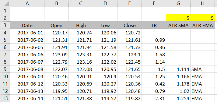
=IF(ROW(F5)<4+H$2,"",IF(ROW(F5)=4+H$2,"SMA","EMA"))Instead of actual calculations, I'm using the placeholders "SMA" and "EMA" for now.
There are two IF functions. The first condition checks whether the current row is smaller than 4 + ATR period. The number 4 corresponds to the first row of our data. For example, if we set ATR period to 5, this condition becomes current row < 4 + 5 and the formula will return "" in all rows above row 9. Starting from row 9, the condition will no longer be true and the next part of the formula will be executed.
The next part is another IF function. This time the condition checks whether the current row is equal to 4 + ATR period. If it is, we will calculate simple moving average (arithmetic average) of true range. If it isn't (therefore it must be greater), we will calculate the EMA ATR formula.
With the placeholders "SMA" and "EMA" and ATR period set to 5, the results look like this:
ATR Formulas
Now we only need to replace "SMA" and "EMA" with the formulas to get the correct results.
The SMA formula is very simple – we can use the formula from the SMA ATR method in the first part of this tutorial. In the formula in cell H5, we will replace "SMA" with this:
AVERAGE(OFFSET(F5,1-H$2,0,H$2,1))Note: Unlike the SMA ATR method, in this case we know the range will always start in row 5, so we could actually use a simpler formula:
AVERAGE(H$5:H5)... and get the same result. Both the formulas above return the same thing when used with the IF condition ROW(F5)=4+H$2.
If you have chosen the first version, the entire formula in cell H5 becomes:
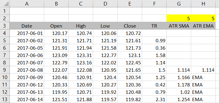
=IF(ROW(F5)<4+H$2,"",IF(ROW(F5)=4+H$2,AVERAGE(OFFSET(F5,1-H$2,0,H$2,1)),"EMA"))You can copy this formula to the other rows to check the results. If you have the IF conditions right and ATR period set to 5, you should see empty cells in rows 5-8, then the number 1.114 (the 5-period SMA ATR) in cell H9, and "EMA" in the rows below.
Let's now replace "EMA" with a new EMA ATR formula:
ATR = a · TR + ( 1 – a ) · ATR1
ATR = ( 2 / ( n +1 ) ) · TR + ( 1 – 2 / ( n + 1 ) ) · ATR1
In the formula in cell H5, we will replace "EMA" with:
2/(H$2+1)*F5+(1-2/(H$2+1))*H4)The entire formula in cell H5 becomes:
=IF(ROW(F5)<4+H$2,"",IF(ROW(F5)=4+H$2,AVERAGE(OFFSET(F5,1-H$2,0,H$2,1)),2/(H$2+1)*F5+(1-2/(H$2+1))*H4))Two things to pay particular attention to are brackets and absolute vs. relative references.
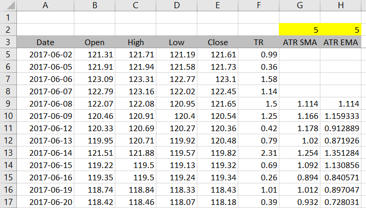
If you copy the formula from H5 to the other rows, you should get these results for ATR period 5 and the GLD daily data we are using:
Wilder's Smoothing Method ATR
The last of the three methods that remains is Wilder's smoothing method. This is the one presented in New Concepts in Technical Trading Systems, the book by J. Welles Wilder that first introduced ATR to the world.
It is in fact almost the same as the EMA ATR method explained above, with just one difference.
Under the EMA method the smoothing factor a is calculated as 2 / ( n + 1). Under Wilder's method it is simply 1 / n. The ATR formula becomes:
ATR = ( 1 / n ) · TR + ( 1 – 1 / n ) · ATR1
Therefore, we can use the formula from the EMA method and only change the smoothing factor to get Wilder's ATR. The formula in cell I5 is:
=IF(ROW(F5)<4+I$2,"",IF(ROW(F5)=4+I$2,AVERAGE(OFFSET(F5,1-I$2,0,I$2,1)),1/I$2*F5+(1-1/I$2)*I4))... where I$2 is the ATR period for this column. The part that has changed from the EMA method is the last part:
1/I$2*F5+(1-1/I$2)*I4The results with our data look like this:
The Best Method and Period
You can see that the three methods give quite different results even with the same period setting. This is not a surprise when you look at the formulas.
You may be wondering which method and which period are the "correct" ones.
Regarding ATR period, popular ones appear to be 14 and 20, but there is no magic number. Consistency and suitability to your particular purpose and conditions are more important than the exact value you choose. Furthermore, discussing the best period doesn't make any sense without also specifying which method we are using, because the period's effect is different across methods. More here.
Regarding the calculation methods, obviously the "correct" method is the one presented by the original author of ATR, J. Welles Wilder. That said, my experience from using various financial or charting software is that all the three methods are commonly used. One problem is that many trading platforms and charting packages lack proper documentation and you don't know which of the methods the particular software is using. This is why it's useful to be able to calculate ATR yourself and compare other party results with your own. This is also the reason that first led me to developing the ATR Calculator.