Calculating Option Strategy Break-Even Points

This is part 8 of the Option Payoff Excel Tutorial. In the previous parts we have created a spreadsheet that calculates P/L of an option strategy, draws payoff diagrams and calculates maximum profit, maximum loss and risk-reward ratio.

In this section we will calculate break-even points – the exact underlying price points where the position's outcome turns from loss to profit and vice versa.

Setting Up Example Option Strategy

We will use an example of iron butterfly position with strikes 45/50/55 – see the screenshot below for details. I have entered the strikes in a rather unusual order on purpose, as we want to make the calculator work regardless of the order of legs that user enters.

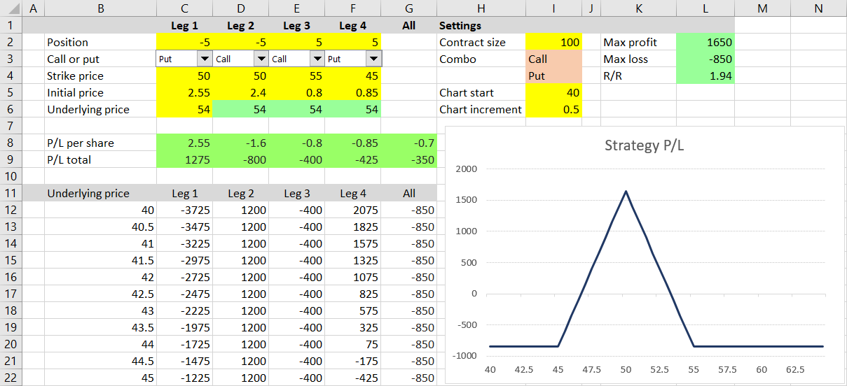
This particular position has maximum profit of $1,650 (cell L2), maximum loss of $850 (cell L3) and risk-reward ratio of 1 : 1.94 (cell L4).

When you look at the payoff diagram, you can see this position probably has two break-even points: one somewhere around 47 and another somewhere around 53 (these are the underlying prices where the blue P/L line crosses zero). Now we will calculate the exact figures.

Payoff Function Properties and B/E Points

We will once again use the payoff function properties which we discussed in part 6. Remember that P/L at expiration as a function of underlying price:

• is always linear (no curves at expiration) and
• its direction or slope can only change at the strikes.

Knowing these helped us find maximum profit and maximum loss in part 6 and it will now help us find the break-even points.

Identifying Key Underlying Price Points

Like we did in part 6, we can identify a number of "important" or "key" underlying price points – all the strikes, zero and infinite. These are the only points where something important (change of P/L slope, maximum or minimum) can occur.

Between each pair of adjacent key points, the P/L function is always a straight line – constant, increasing or decreasing. This also means that there can't be more than one break-even point between each pair of adjacent key points. There is always either one B/E or none.

For a strategy with three different strikes, as we have in our example – 45/50/55, we have five key points:

• Zero
• The 45 strike
• The 50 strike (two legs have this strike in our case)
• The 55 strike
• Infinite

These points divide the entire range of possible underlying prices into four "sections".

Deciding If There Is a B/E

To find out whether there is a break-even point in a particular section between two points, we only need to know whether the P/L at these points is positive or negative.

If the signs are different (one P/L positive and the other negative), the P/L line must cross zero somewhere between the two points and there is a break-even. If the signs are the same, there is no B/E. We will use this logic for our Excel calculations.

Excel Implementation

We will make these calculations at the bottom of our sheet, below the chart's X-axis and maximum profit and loss calculations. We can copy the column labels from row 63 to row 72.

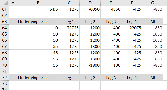
Although we have already worked with the key points in part 6 when calculating maximum profit and maximum loss, so we can find them in rows 64-70, now we also need them sorted from lowest to highest (in order to know the adjacent pairs). Therefore it is best to start our calculations over from the beginning.

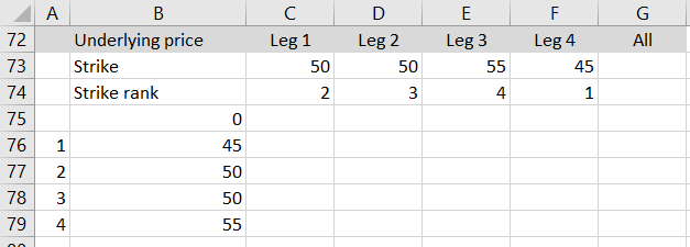
The first task is to identify the strikes and order them from lowest to highest.

First let's get all the strikes in row 73. We want cells C73-F73 to display the strike for the particular leg (the same number as in row 4 – the strike input cells), but only if this particular leg is being used for the current strategy (position size in row 2 is not zero). For positions with fewer than four legs, some of the four columns are not used (position size zero), but may still have numbers in the strike input cells (we don't want to rely on the user to always delete the strike inputs when not using the particular column). We want row 73 to display zero for these inactive legs.

In other words, we want cell C73 to display the first leg strike (cell C4) if position size (cell C2) is not zero, and display zero if position size is zero.

The formula in cell C73 is:

=IF(C2=0,0,C4)

... using the familiar IF Excel function.

Make sure you have relative references to C2 and C4 (no dollar signs) and copy the formula to the other legs – to cells D73, E73, F73.

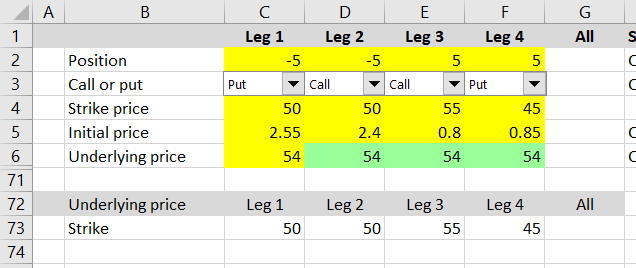
Test it by changing some of the position sizes in row 2 to zero – row 73 should also change to zero.

Ranking the Strikes

In the next row we will rank the strikes from lowest to highest. We can use the Excel function RANK.EQ (RANK in Excel 2007 and earlier). The formula in cell C74 is:

=RANK.EQ(C73,$C$73:$F$73,1)

... where:

• C73 is the cell which we want to rank (the current leg strike, with relative reference)
• $C$73:$F$73 is the range of all the values (all the strikes, with absolute references, because the range will be the same for all the legs)
• 1 means we want the rank ascending (lowest strike gets rank 1)

Copy the formula to cells D74, E74, F74 and you should see this:

You can see that when there are duplicate values (strike 50 in our example), the RANK.EQ function returns the same rank (the lowest) for all of them. But in this case we want to make the ranks unique (we want one of the 50 strikes to have rank 2 and the other to have rank 3) and adjust the formula in C74 like this:

=RANK.EQ(C73,$C73:$F73,1)+COUNTIF($C73:C73,C73)-1

The first half is the same. We have added the COUNTIF function, which returns the count of cells in a given range ($C73:C73) which are equal to the value in the second parameter (C73). For example, if you have a range of numbers 10, 30, 20, 30, 10 and ask how many times the value 30 is in that range, the function would return 2. In this case, for leg 1 the COUNTIF returns 1 (because we are asking how many times the value of cell C73 is in cell C73, which of course is once). Because we also have the -1 at the end of the formula, the resulting rank does not change in this case and it is still 2.

Make sure you have the dollar sign right in the $C73:C73 part and copy the formula from cell C73 to cells D73, E73, F73.

You should get the ranks 2, 3, 4, 1. The one rank which has changed is the rank of the second 50 strike, which has increased from 2 to 3. This was done by the COUNTIF function, which asked how many times the value 50 is in cells C73 and C74. It is 2 times, so COUNTIF returns 2. Combined with the -1 at the end, the new rank is higher by 1 compared to the ranks we had without the COUNTIF previously.

Listing Ordered Key Points

Now we have the strikes ranked from 1 to 4 and each strike has a unique rank. We have everything ready to list all our key underlying price points, ordered from zero to the highest strike in cells B75 to B79.

Put the value zero in cell B75.

Cells B76 to B79 will be strikes with rank 1 to 4, in this order. Put the numbers 1, 2, 3, 4 in cells A76, A77, A78, A79, respectively.

Cell B76 should be the lowest strike = the strike with rank 1 (this is why we put the number 1 in cell A76).

The formula in cell B76 should perform two tasks:

1. Find out, which of the legs has strike with rank 1.
2. Return the strike for that leg.

The Excel function which can do the first task is MATCH. We will use it to find out, where in the range of cells C74-F74 is the value 1. The function takes three parameters and the syntax is:

=MATCH(value we are looking for, range where we are searching, type of match)

In our case:

=MATCH(A76,$C$74:$F$74,0)

... where:

• A76 is the cell where we have put the desired rank (the number 1)
• $C$74:$F$74 is the range of cells where we are looking for the number 1
• 0 denotes exact match

The function will return the value 4 in our example, because the value we are looking for (1) is in cell F74, which is the fourth cell in the range C74-F74.

Now we will do the second part – get the strike price for the leg whose number we have just found with MATCH (leg 4). We are asking the question: What is the value of the 4th cell in the range C73-F73?

We will use the INDEX function with two parameters: the range where our strikes are (C73-F73) and the position of the cell we are looking for (the number 4 which we have found with MATCH). The syntax is:

=INDEX(range, position)

=INDEX(the cells with strikes, the output of MATCH)

=INDEX($C$73:$F$73,MATCH(A76,$C$74:$F$74,0))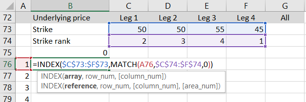

Copy the formula from cell B76 to cells B77, B78, B79 to get the strikes with ranks 2, 3, 4, respectively. The result should look like this:

Note: This INDEX-MATCH combination is very useful and popular. Together with VLOOKUP and HLOOKUP it is the core of Excel lookup functions, which enable you to do a lot of powerful things with large datasets. These functions are worth mastering, not only for the purpose of this tutorial.

We have now listed zero and the four strikes, ordered from lowest to highest, and we have one last key point to add – the infinite underlying price. In cell B80, we won't actually enter infinite, but some very large number (so large you are sure all your possible strikes and break-evens for any underlying and any option strategy will be smaller than this number). I choose 1,000,000,000 (one billion).

Calculating P/L

Now we have all the six key points (duplicates are fine, as long as all the key points are ordered from lowest to highest). We can calculate the position's P/L at each point, simply by copying the formulas from cells C70-G70 (or any of the other rows which calculate P/L for given underlying price) to rows 75-80. The result should look like this:

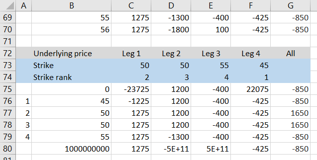
I have colored the background of rows 73-74 just to remember these formulas are different than the other rows.

Finding Break-Even Points

The next step is to find where (between which of the adjacent key points) the break-evens are. As explained in the beginning, we will do this by comparing the signs of the P/L's for the two points. If the sign is different, we know there is a B/E between them. If sign is the same, no B/E. Just by looking at the P/L's in column G, we can see there should be a break-even point between 45 and 50 (P/L goes from -850 to +1,650) and another one between 50 and 55 (P/L goes from +1,650 to -850).

Let's do it with Excel formulas in column H, next to the calculated P/L. We will check for B/E's in each of the five possible intervals, starting with the one between zero and the first strike.

The formula in cell H76 is:

=IF(SIGN(G76)=SIGN(G75),0,1)

It is a very simple IF function that checks whether the P/L signs are the same (both are profits or both are losses). If they are the same, it returns zero (no B/E). If they are not the same, it returns 1 (there is a B/E somewhere between these two underlying price points).

Copy the formula from cell H76 to cells H77-H80. You should have this result:

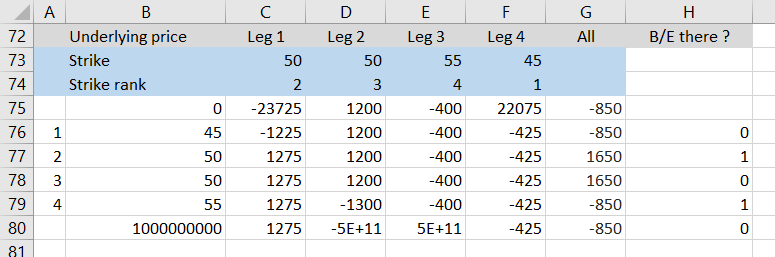
The calculations have confirmed what we were thinking just by looking at the payoff chart and the P/L's. There are two break-even points: one between 45 and 50, another between 50 and 55.

You can also see that the strike 50 being included two times doesn't matter, because P/L at identical underlying prices is of course the same (+1,650), therefore the signs are the same, which means no false break-evens are found.

Now that we know where to look for B/E points, we can calculate the exact prices.

Calculating the Exact Break-Even Prices

We know that the P/L at expiration as function of underlying price is always a straight line between two adjacent strikes and therefore we can calculate the exact underlying price where P/L crosses the zero line by interpolating. Let's do that for the B/E point between strikes 45 and 50.

We know that at strike 45 total P/L is -850 and at strike 50 it is +1,650. We also know the line between these two points is straight, with constant slope. Therefore, the ratio of the break-even point distances from the two strikes x₁ : x₂ must be equal to the ratio of distances between zero and the two P/L's y₁ : y₂.

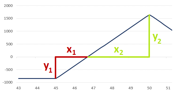
Knowing this, we can calculate the distance of the break-even point from the lower strike:

x₁ = (x₁ + x₂) * y₁ / (y₁ + y₂)

... where

• x₁ + x₂ is the distance between strikes = 50 – 45 = 5 in our example
• y₁ is zero minus the lower strike P/L = 0 – (-850) = 850
• y₁+y₂ is the higher strike P/L minus the lower strike P/L = 1650 – (-850) = 2500

Therefore:

x₁ = 5 * 850 / 2500 = 1.7

The break-even point is:

45 + 1.7 = 46.70

Let's implement this calculation in Excel in cell I77. The formula is:

=B76+(B77-B76)*(0-G76)/(G77-G76)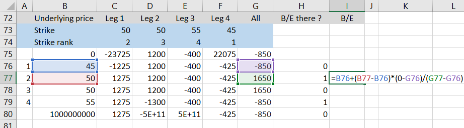

Before copying the formula to the other cells, let's make it only calculate the B/E price if there is one in the particular interval (if column H is 1). We will do this by putting the entire formula inside a simple IF function that will check the value in column H:

=IF(H77=0,0,B76+(B77-B76)*(0-G76)/(G77-G76))

Now we can copy cell I77 to cells I76 and I77-I79. The result should look like this:

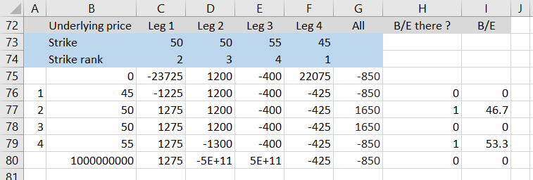
The second break-even point is 53.30.

That's It (Almost)

We have successfully calculated break-even points, which was the last feature to add to our strategy payoff spreadsheet. We are approaching the end of the Option Payoff Excel Tutorial, but there is one last part where I will introduce a few more ideas and possible further improvements to our spreadsheet.

Go to the last part: Further Improvements